Analysis on {0,1}^N

The set \{0,1\}^{\mathbb{N}}, where \mathbb{N} is the set of natural numbers, consists of infinity strings of zeros and ones. It is equipped with mod(2) addition structure and it is called Cantor group, or dyadic group. Another notation is \prod_{1}^{\infty} \mathbb{Z}/2\mathbb{Z}. One studies functions f : \{0,1\}^{\mathbb{N}} \to \mathbb{R}.

One question one can ask is why historically we started with f : [0,1) \to \mathbb{R} and not with f : \{0,1\}^{\mathbb{N}} \to \mathbb{R}? Is not from the prospective of computers functions on \{0,1\}^{\mathbb{N}} more convenient to use? I understand that there is a binary correspondence (not necessarily unique) between [0,1) and \{0,1\}^{\mathbb{N}} but one may forget what kind of structures we had on \{0,1\}^{\mathbb{N}} after we moved to [0,1)? In egeneral we can encode everything via zeros and ones but we may lose symmetries and structures that we had on one side when we moved to the other side. So why nowadays we start teaching Fourier analysis on C([0,2\pi), dx) and not on \{0,1\}^{\mathbb{N}} equipped with a uniform measure (I will explain below what is meant by uniform measure on \{0,1\}^{\mathbb{N}})?

I do not have complete answers to these questions, perhaps Zygmund’s beautiful book on trigonometric series had a nontrivial influence on historical development of Fourier analysis on [0,2\pi).

In this post I will try briefly talk about Fourier analysis on \{0,1\}^{\mathbb{N}}. I saw a question on mathoverflow asking what harmonic analysis we have on \{0,1\}^{\mathbb{N}}. I wrote the answer there, and I thought I would share it here as well.

Harmonic analysis on \{0,1\}^{\mathbb{N}} can be different depending on how one enumerates orthonormal basis, so called Walsh functions.

One usually considers Haar measure dm on \{0,1\}^{\mathbb{N}} which is a probability measure in the following sense: if you have a function f :\{0,1\}^{\mathbb{N}} \to \mathbb{R} which depends only on the first n variables, say f(x_{1}, ...) =g(x_{1}, \ldots, x_{n}) then

\begin{aligned} \int_{\{0,1\}^{\mathbb{N}}} f(x)dm(x) = \frac{1}{2^{n}} \sum_{(x_{1}, \ldots, x_{n}) \in \{0,1\}^{n}}g(x_{1}, \ldots, x_{n}). \end{aligned}

Orthonormal system on L^{2}(\{0,1\}^{\mathbb{N}}, dm) is called Walsh system, and perhaps it was first time introduced by Walsh in 1923: this is a certain family of functions on \{0,1\}^{\mathbb{N}} taking values +1 or -1.

I have seen 4 different enumerations of this family of functions used in the literature (perhaps there are more). The first 3 of them (original Walsh, Paley, and Walsh–Kaczmarz) is well described in the book F. Schipp, WR. Wade, P. Simon, “Walsh series: an introduction to dyadic harmonic analysis”, see Section 1.4. The 4th one which I find kind of exceptional is not there.

1). Walsh’s original enumeration: Walsh defined his system recursively. Later, it turned out that they can be written as follows:

\begin{aligned} \varphi_{n}(x) = (-1)^{\sum_{k=0}^{\infty}(n_{k}+n_{k+1})x_{k+1}}, \quad n \in \mathbb{N}, \end{aligned}

where n=\sum_{k=0}^{\infty} n_{k} 2^{k} with n_{k} \in \{0,1\}, and x=(x_{1}, \ldots ) \in \{0,1\}^{\mathbb{N}}. In other words (n_{0}, n_{1}, \ldots) is the binary representation of the positive integer n. The system \{\varphi_{n}(x)\}_{n\geq 1} is the Walsh’s original system.
Partial sums S_{m}f = \sum_{k=0}^{m} c_{k} \varphi_{k}, where c_{k} = \int_{\{0,1\}^{\mathbb{N}}}f \varphi_{k} dm, converge to f in L^{p}, p>1. The latter is equivalent to the statement that

\begin{aligned}\sup_{n \geq 1}\| S_{n} f\|_{p} \lesssim \|f\|_{p}, \quad 1<p<\infty \end{aligned}.

Moreover S_{n} f converges to f for any f \in L^{p}(\{0,1\}^{\mathbb{N}}, dm) provided that p \in (1,\infty). This is a consequence of Carleson’s maximal inequality

\begin{aligned} \| \sup_{n \geq 1} |S_{n} f| \|_{p} \lesssim \|f\|_{p}, \quad 1<p<\infty. \end{aligned}

Luzin asked in the trigonometric case on the unit circle \mathbb{T}. Carleson proved for p=2; Hunt extended to 1<p<\infty. Billard proved for the original Walsh system for p=2; Sjölin extended for 1<p<\infty.
Fejer means are bounded, i.e.,

\begin{aligned} \sup_{n\geq 1}\left\| \frac{S_{1}+...+S_{n}}{n} f\right\|_{p} \lesssim \|f\|_{p}, \quad 1\leq p \leq \infty \end{aligned}

In the book F. Schipp, WR. Wade, P. Simon, there is a more “martingale proofs” of these results. Dyadic martingales naturally appear here. For example, \{ S_{2^{k}}f\}_{k \geq 0} is a martingale. In fact,
S_{2^{k}}f = \mathbb{E} (f | \mathcal{F}_{k}), where \mathcal{F}_{k} is \sigma-algebra, which is generated by atoms, where atoms are I_{k}(x) = \{ y \in \{0,1\}^{\mathbb{N}} : y_{1}=x_{1}, \ldots ,y_{k}=x_{k}\}. In probabilistic language you condition on the first k variables, and let the tail be the everything. Then, for example, the statement that

\begin{aligned} \|\sup_{k \geq 0}|S_{2^{k}} f|\|_{p} \lesssim \|f\|_{p} \quad 1<p<\infty \end{aligned}

is exactly Doob’s maximal inequality. The book F. Schipp, WR. Wade, P. Simon, “Walsh series: an introduction to dyadic harmonic analysis” provides more martingale techniques. The paper A guide to Calreson’s theorem by Ciprian Demeter has more time-frequency analysis introduction.

  1. Paley’s enumeration (Walsh–Paley functions). In 1932, Paley proposed a different enumeration of Walsh functions

    \begin{aligned} w_{n}(x) = (-1)^{\sum_{k=0}^{\infty} n_{k}x_{k+1}}, \quad n \in \mathbb{N}. \end{aligned}

    Paley’s enumeration perhaps is more close to the classical trigonometric system \sin(ns) and \cos(ns). We can “identify” [0,1) with \{0,1\}^{\mathbb{N}} as follows:

    \begin{aligned} s \in [0,1), \quad s = \sum_{k=1}^{\infty} s_{k} 2^{-k} \end{aligned}

    for some s_{k} \in \{0,1\}. This identification is not unique, for example, \frac{1}{2^{2}} can be written as (0,1,0,0,\ldots) and also as (0,0,1,1,1\ldots,). Among these two one choose the first one, i.e., when number of 1’s terminate starting from some place. Such bad points are not too many, they have zero measure so we do not bother with them. In particular \omega_{n}(s) is defined for s \in [0,1). Then

    \begin{aligned} w_{2^{k}}(s) = (-1)^{s_{k+1}} =\mathrm{sign}(\sin(2^{k+1} \pi s)) \approx \sin(2^{k+1} \pi s), \quad s \in (0,1]. \end{aligned}

    In general, \omega_{n}(s) is close to \sin(ns) or \cos(ns) depending n is even or odd.
    Frequencies \sin(2^{k+1} \pi s) are independent pretty much in the same way as \omega_{2^{k}}(s) = (-1)^{s_{k+1}} are independent: Khinchin’s inequality holds for both of them \| \sum c_{k} \omega_{2^{k}} \|_{2} \asymp \| \sum c_{k} \omega_{2^{k}} \|_{1}, and \| \sum c_{k} \sin(2^{k+1} \pi s) \|_{1} \asymp \| \sum c_{k} \sin(2^{k+1} \pi s)\|_{2}.
    One has the notion of “dyadic derivative”

    \begin{aligned} df(x) = 2^{0} \frac{f(x_{1}, x_{2}, \ldots) - f(1-x_{1}, x_{2}, \ldots)}{2}+2^{1}\frac{f(x_{1}, x_{2}, \ldots) - f(x_{1},1-x_{2}, \ldots)}{2}+2^{2} \ldots \end{aligned}

    provided that the sum converges. Perhaps one should call it “dyadic Laplacian” instead of the derivative. One can verify that Walsh–Paley functions are eigenfunctions: d\omega_{n}(x) = n \omega_{n}(x). One can study polynomials of degree m, say finite sums x \mapsto \sum_{k=0}^{m} c_{k}\omega_{k}(x), and ask questions similar to Markov–Brother’s and Bernstein estimates for such polynomials. One can ask regularity questions: if f is regular on (0,1] how regular it is on \{0,1\}^{\mathbb{N}} with respect to dyadic derivative and vice versa. What happens with partial sums if we have some regularity in terms of dyadic derivatives etc. The results about L^{p} convergence of partial sums, Carleson–Hunt theorem also hold for this enumeration.

  2. Sneider’s enumeration (Walsh-Kaczmarz system) was introduced by Sneider:

    \begin{aligned} k_{0}(x) =1, \quad k_{n}(x) = (-1)^{x_{A}+\sum_{k=0}^{A-1} n_{A-k-1}x_{k+1}}\quad \text{where} \quad 2^{A}\leq n < 2^{A+1} \end{aligned}

    I won’t say much about this system except that the same L^{p} convergence theorems hold in this case. Perhaps an interesting observation in all these 3 enumerations is that Dirichlet Kernels
    D_{n}(x) = \sum_{k=0}^{n-1} a_{n}(x) where a_{n} is either Walsh, Walsh–Paley, Walsh–Kaczmarz, for n=2^{k} are the same. In fact D_{2^{k}}(x) =\prod_{j=1}^{k}(1+(-1)^{x_j}).

Frequencies: when working with these 3 enumerations one usually thinks that a_{n}(x) is “high-frequency” element if n is large, and “low-frequency” element if n is small. For example \omega_{2^{k}}(x) = (-1)^{x_{k+1}} for large k are high frequency elements similar to \sin(2^{k+1}\pi s). All these 3 enumerations and concepts of frequencies tend to mimic the harmonic analysis on L^{p}(\mathbb{T}, d\theta), where d\theta is the uniform measure on the unit circle, i.e., trigonometric polynomials.

  1. Probabilistic enumeration (from independent towards dependent). In this enumeration the concept of “high/low frequencies” is changed in a very opposite way. In fact, the elements \{ \omega_{2^{k}}(x)\}_{k \geq 0} will be the lowest frequencies, say frequencies of degree 1. Elements \omega_{n}(x) where n has two bits in its binary representation will be frequencies of order 2. These are precisely Walsh functions (-1)^{x_{i}+x_{j}}, i<j. In a certain sense enumeration starts from “independent frequencies to dependent ones“, and probabilistic ideas, measure concentration phenomena, dimension independent phenomena, and the concept of “independence” happen to be useful. The goal is to represent functions f : \{0,1\}^{\mathbb{N}} \to \mathbb{R} as follows:

    \begin{aligned} f(x_{1},x_{2}, \ldots) = c_{0} + \underbrace{c_{1}(-1)^{x_{1}}+c_{2}(-1)^{x_{2}}+\ldots+c_{i}(-1)^{x_{i}}+\ldots}_{\mathrm{linear\; terms}} \end{aligned}
    \begin{aligned}+\underbrace{c_{12}(-1)^{x_{1}+x_{2}}+c_{13}(-1)^{x_{1}+x_{3}}+\ldots+c_{ij}(-1)^{x_{i}+x_{j}}+\ldots}_{\mathrm{second\, order\, terms}}+\mathrm{higher\, order \, terms} \end{aligned}

    Of course, if one takes f \in L^{2}(\{0,1\}^{\mathbb{N}}, dm), writes into Walsh–Paley system f(x) = \sum_{n\geq 0} a_{k} \omega_{k}(x), and wants to rearrange the terms to write in the form (1) then rearranged infinity sums may give different results unless \sum |a_{n}| <\infty which is very unlikely for a “typical” f \in L^{2}. However, if one considers functions f which depend only on the first n variables the rearranged sums will be the same. This is not a big restriction on the class of functions because when one wants to prove a statement for functions on \{0,1\}^{\mathbb{N}} one does not start with f \in L^{2} which depends on all its variables, one starts from a “finite dimensional problem” when f depends only on the first n variables, and one proves the corresponding statements for such functions, requires the constants involved in the statement to be independent of n, and then passes to a limit, i.e., to an infinite dimensional problem.
    Thus if we consider functions f which depend only on the first n variables then

    \begin{aligned} f(x_{1}, \ldots, x_{n}) = c_{0}+c_{1}(-1)^{x_{1}}+\ldots +c_{n}(-1)^{x_{n}}+\sum_{1\leq i<j \leq n} c_{ij}(-1)^{x_{i}+x_{j}} + \ldots  = \sum_{S \subset \{1, \ldots, n\}} a_{S}\, (-1)^{\sum_{j \in S} x_{j}} \end{aligned}

    The latter notation seems to be compact and convenient. Here a_{S} are Fourier coefficients, and (-1)^{\sum_{j \in S} x_{j}} are Walsh functions (enumerated in a strange way) indexed by the sets S. Since this enumeration works well provided that f depends only on finite number of variables, the questions about L^{p} convergence, Carleson–Hunt theorem etc do not make any sense. So the direction of harmonic analysis in which Luzin was interested ends here. Well, one can still consider partial sums

    \begin{aligned} S_{d} f (x) = \sum_{\substack{S \subset \{1, \ldots, n\}\\ |S|\leq d}} a_{S} \, (-1)^{\sum_{j \in S} x_{j}}, \end{aligned}

    where |S| denotes the cardinality of the set S, and ask similar questions

    \begin{aligned} \| S_{d} f\|_{p} \lesssim \|f\|_{p} \end{aligned}

    with uniform bound for all d, 1\leq d \leq n, for all n\geq 1, and all f depending on the first n variables. Such estimate holds if and only if p=2.
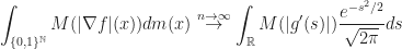
    Interesting connection arises with Gauss space. For example

    \begin{aligned} \frac{\ell!}{n^{\ell/2}} \sum_{\substack{S \subset\{1, \ldots, n\}\\ |S|=\ell}} (-1)^{\sum_{j \in S} x_{j}} \stackrel{d}{\to} H_{\ell}(\xi) \end{aligned}

    where H_{\ell} is degree \ell probabilists’ Hermite polynomial, \xi \in \mathcal{N}(0,1) is the standard normal Gaussian random variable, and the convergence is in the sense of distributions. By Taking tensor products of the above example one recovers Hermite polynomials on \mathbb{R}^{N} with arbitrary N. So, because of this limit, it is reasonable to think about (-1)^{\sum_{j \in S} x_{j}} as low frequency element if |S| is small, and high frequency element if |S| is large (which is very opposite compared to the original Walsh enumeration). In fact, the analysis with such enumeration (1) for functions f depending on n variables is similar to the one on L^{p}(\mathbb{T}^{n}, d\theta^{n}). Dscrete Laplacian is defined in a different way

    \begin{aligned} \Delta f(x) = \sum_{j=1}^{n} D_{j}f(x), \end{aligned}

    where D_{j}f(x_{1}, \ldots, x_{n}) = \frac{f(x_{1}, \ldots,x_{j}, \ldots, x_{n})-f(x_{1}, \ldots, 1-x_{j}, \ldots, x_{n})}{2}. One also considers discrete gradient

    \begin{aligned} Df(x) = (D_{1} f(x), \ldots, D_{n}f(x)). \end{aligned}

    One has integration by parts formula

    \begin{aligned} \int_{\{0,1\}^{\mathbb{N}}} g \Delta f dm=\int_{\{0,1\}^{\mathbb{N}}} Df \cdot Dg\, dm \end{aligned}

    for all functions f,g depending on the first n variables. Heat semigroup

    \begin{aligned} e^{-t\Delta} f = \sum_{S \subset \{1, \ldots, n\}}a_{S} e^{-t|S|} (-1)^{\sum_{j\in S}x_{j}} \end{aligned}

    satisfies heat equation \frac{\partial }{\partial t} e^{-t\Delta}f = -\Delta e^{-t\Delta}f. Discrete gradient

    \begin{aligned} |\nabla f|(x) = \sqrt{\sum_{j=1}^{n} |D_{j}f(x)|^{2}} \end{aligned}

    when applied to f(x_{1}, \ldots, x_{n}) = g\left(\frac{(-1)^{x_{1}}+\ldots+(-1)^{x_{n}}}{\sqrt{n}}\right) for some smooth bounded g :\mathbb{R} \to\mathbb{R}, converges to the classical derivative

    \begin{aligned} \int_{\{0,1\}^{\mathbb{N}}} M(|\nabla f|(x)) dm(x) \stackrel{n \to \infty}{\to} \int_{\mathbb{R}}M(|g'(s)|) \frac{e^{-s^{2}/2}}{\sqrt{2\pi}}ds \end{aligned}

    for any smooth functions M. The case M(t)=|t|^{p} is a typical application. Denoting (-1)^{x_{j}} = \varepsilon_{j}, then \ell degree polynomials with respect to this enumeration can be written as

    \begin{aligned} g(\varepsilon_{1}, \ldots, \varepsilon_{n}) =\sum_{\substack{S \subset \{1, \ldots, n\} \\ |S|\leq \ell}} a_{S} \prod_{j \in S} \varepsilon_{j} \end{aligned}

    and the latter expression can be extended in a natural way for all \varepsilon_{1}, \ldots, \varepsilon_{n} \in \mathbb{R} as a multilinear classical polynomial in n variable of degree d. Due to the identity \|g\|_{L^{\infty}([-1,1]^{n})} = \|g\|_{L^{\infty}({-1,1}^{n})} tools from approximation theory enter in an unexpected way applied to actual degree \ell multilinear polynomials. Discrete derivatives coincide with the actual derivatives for such multilinear polynomials. Boolean functions f :\{0,1\}^{\mathbb{N}} \to \{0,1\} have an extra property f^{2}=f and this gives more cancelations when proving statements for all real valued functions.

To summarize: Harmonic analysis on \{0,1\}^{\mathbb{N}} depends on how one encodes Walsh functions, i.e., frequencies in the Hilbert space L^{2}(\{0,1\}^{\mathbb{N}}, dm), who are the low and who are the high frequency functions.

Design a site like this with WordPress.com
Get started